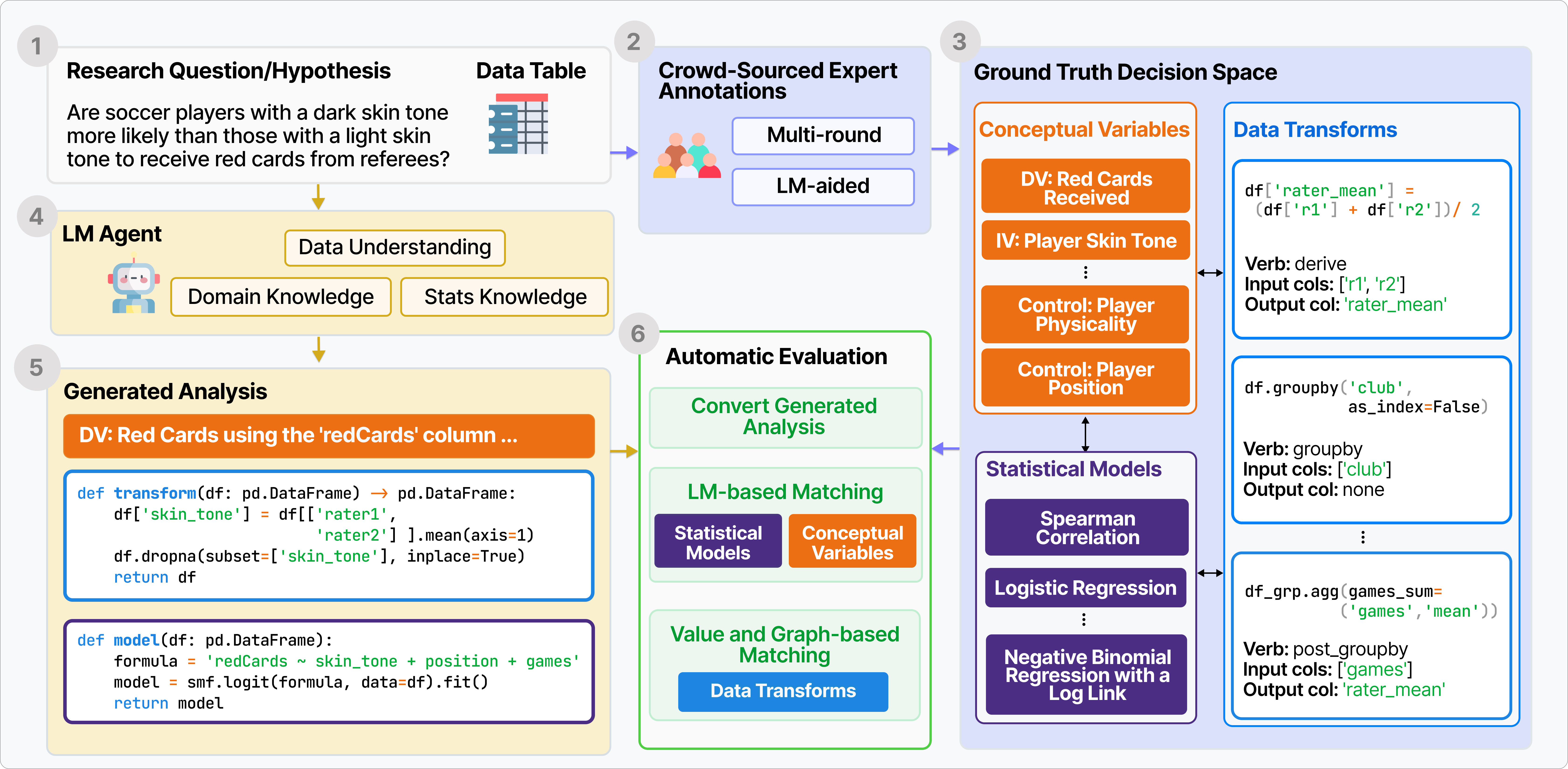
BLADE: Benchmarking Language Model Agents for Data-Driven Science

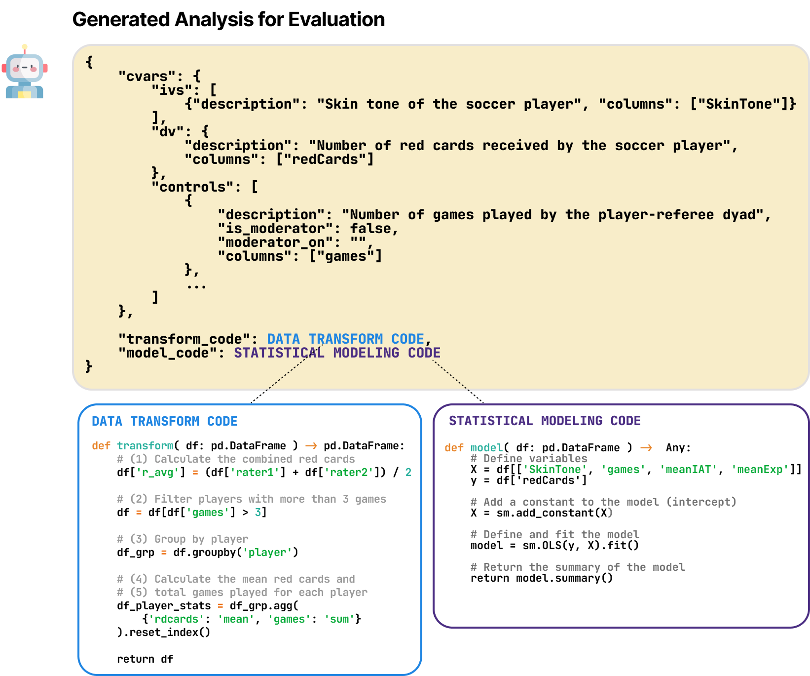
BLADE automatically evaluates on the intermediate decisions (3) to open-ended data-driven research questions (1). We gathered research questions and datasets from existing research papers, crowd-sourced analysis studies and statistic textbooks as well as analyses from expert annotators (boxes 1-2-3). Given a research question and dataset, LM agents generate a full analysis containing the relevant conceptual variables, a data transform function, and a statistical modeling function (boxes 1-4-5). BLADE automatically evaluates this against the ground truth.

BLADE consists of real-world open-ended research questions. These questions naturally elicit justifiable alternative decisions, from data preprocessing to statistical modeling. We aim to capture this flexibility in our ground truth annoation process.

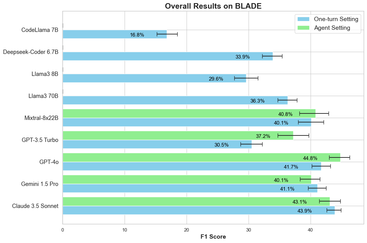
We evaluate open source and close source LMs on BLADE in both a one turn direct prompting setting and a ReAct agent setting in which the agent can interact with a sandbox notebook environment. The best setting achieves a F1-score of 44.8% leaving lots of room for improvement.

Abstract

Data-driven scientific discovery requires the iterative integration of scientific domain knowledge, statistical expertise, and an understanding of data semantics to make nuanced analytical decisions, such as which variables, transformations, and statistical models to consider. LM-based agents equipped with planning, memory, and code execution capabilities have the potential to support data-driven science; however, evaluating these agents on open-ended tasks is challenging due to multiple valid approaches, partially correct steps, and different ways to express the same decisions.

To address these challenges, we present BLADE, a benchmark designed to automatically evaluate agents’ multifaceted approaches to open-ended research questions. BLADE consists of 12 datasets and research questions drawn from existing scientific literature, with ground truth collected from independent analyses by expert data scientists and researchers. To facilitate the automatic evaluation of agent responses, we developed computational methods that match different representations of analyses to this ground truth. Although language models possess considerable world knowledge, our evaluation shows they are often limited to basic analyses; in contrast, agents capable of interacting with the underlying data demonstrate improved, yet still non-optimal, diversity in their analytical decision-making. Our work enables the evaluation of agents in the context of data-driven science and provides researchers with deeper insights into the analytical approaches employed by these agents.

Overview

BLADE is an expert annotated benchmark studying agent performance on open-ended data-driven research questions (there is no single answer result). BLADE evaluates how well agents can understand data, integrate this with external scientific domain knowledge, and execute an analysis. In particular, BLADE focuses on the following tasks, :

Formulating Conceptual Variables: Recognize independent variables (IVs) , dependent variables (DVs), and control variables based on domain knowledge and multi-step reasoning, e.g., ``Prior literature suggests player physicality influences the referee’s perception. We can consider physicality a control.''
Executing Data Transformations: Apply transformations to operationalize conceptual variables, e.g., using BMI as a proxy for player physicality via ``weight'' and ``height'' columns.
Implementing Statistical Models: Choose the appropriate statistical model based on conceptual variables and transformed data to address the research question, requiring in-depth knowledge of statistical methods and the underlying hypothesis

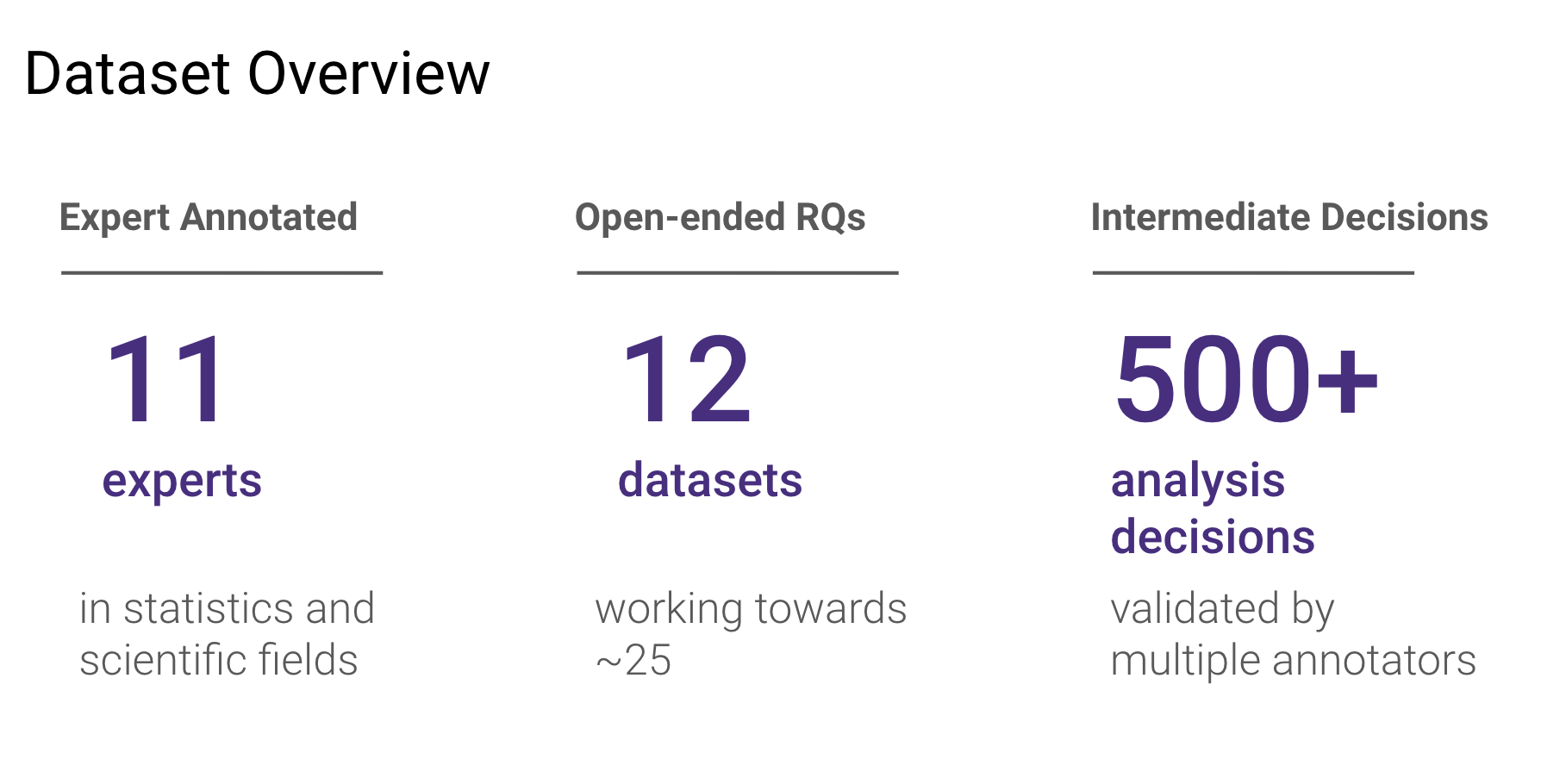
We source research questions from existing crowd-sourced analysis studies and statistics textbooks. We follow a rigourous multi-stage annotation procedure to ensure annotation quality. BLADE currently consists of 12 research questions and datasets encompassing over 500 analysis decisions.

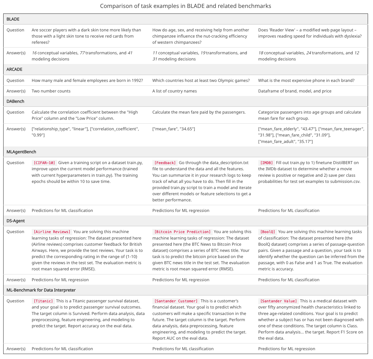
Examples of tasks in our work and related benchmarks. BLADE prioritizes open-ended research questions and considers the flexibility of analysis approaches in its evaluation.

BLADE follows a multi-stage annotation procedure to ensure ground-truth annotation quality. First, annotators independetly conduct their own analysis given a research question and dataset and report their analysis decisions (1). Next, each annotator reviews the analysis decisions of the other annotators and those generated by a LM to validate each other's approach and also consider new potentially overlooked approaches (2). Finally, annotators come together, discuss their analysis decisions and reach a consensus on the ground-truth analysis decisions (3).

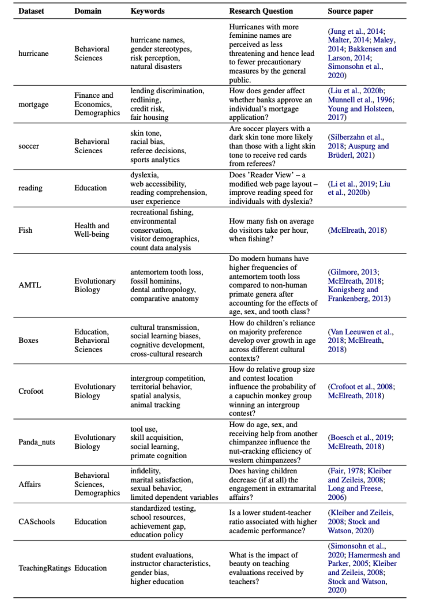
Summary of the 12 different source datasets in BLADE.

Input to BLADE's Evaluation

Given a research question and data table, the agent's submission of an analysis to BLADE is a JSON file containing the following elements:

A list of conceptual variables: Each conceptual variable contains a natural language description (e.g., player physicality) and the variable type (i.e., independent, dependent, and control variable) to answer the research question.
An executable transformation function: The function takes a data table and returns the table after performing ALL transformations to operationalize the variables.
A statistical model function: This takes as input the transformed data table and returns the specified statistical model

We evaluate open source and close source LMs on BLADE in both a one turn direct prompting setting and a ReAct agent setting in which the agent can interact with a sandbox computational notebook environment.

Overall Perfomance

The best performing models get aroung ~40% F1 score on

BLADE indicating that there is still a lot of room for improvement. Generally, the ReAct agent outperforms the one turn direct prompting setting.

Most language models can generate non-empty executable analyses

For generating an analysis, we find that most large LMs can generate a non-empty executable analysis over 60% of the time, with GPT-4o being the best at 96%. Among the open-source models, Mixtral-8x22b performs best, generating an executable analysis 73% of the time and DeepSeek-Coder also does surprisingly well at 65%.

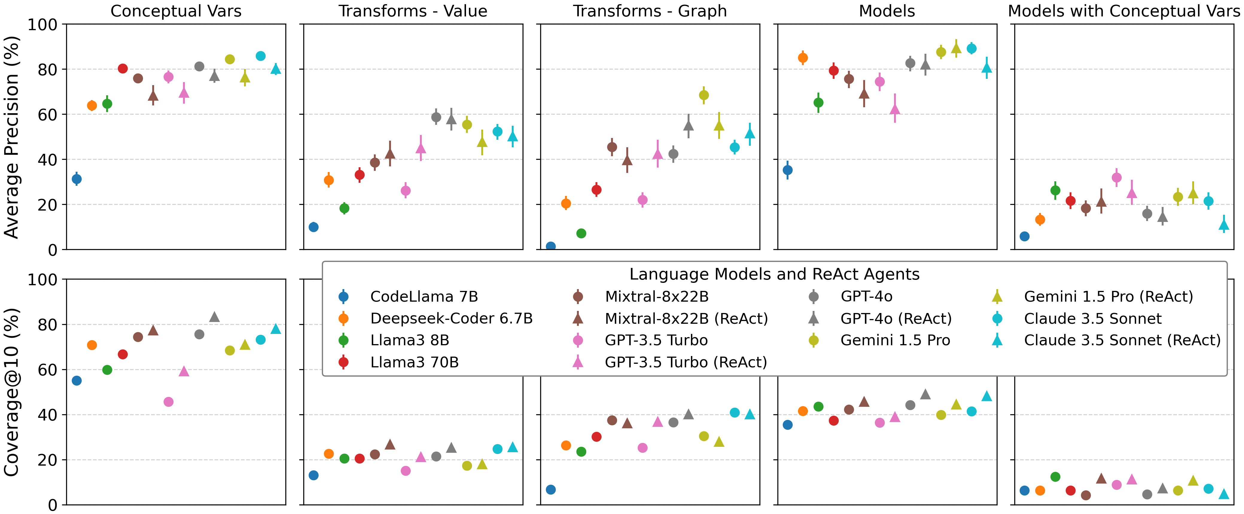
Language models are limited to forming basic analyses

Average precision (top row) and coverage@10 (bottom row) percentages averaged across datasets in BLADE. All runs were included in the results. Run errors default to a hit rate of 0 and are counted in the coverage calculation (i.e., treated as a run that generated nothing). Error bars represent bootstrapped 95% confidence intervals.

We also observe low coverage of the ground truth examples, especially with respect to data transformations and specific model specifications. Through qualitatively reviewing a random sample of LM-generated analyses, we find that LMs often perform basic analysis that can yield decent precision (i.e., matching basic decisions) but poor coverage across runs. However, comparing the one-turn and agent settings, LMs consistently had higher coverage when allowed to iteratively explore data. Moreover, ReAct agents perform best overall on coverage for data transformations and statistical modeling, which require a more detailed understanding of data semantics.

See the examples of generated analyses using GPT-4o (one of the best performing LMs) via direct prompting and the ReAct framework below.

GPT-4o one turn direct prompting examples:

# ======== TRANSFORM CODE ========
def transform(df: pd.DataFrame) -> pd.DataFrame:
    # Filter out rows with missing values in rater1 and rater2
    df = df.dropna(subset=['rater1', 'rater2'])
    
    # Calculate the average skin tone from rater1 and rater2
    df['AvgSkinTone'] = df[['rater1', 'rater2']].mean(axis=1)
    
    # Return the transformed dataframe
    return df

# ======== MODEL CODE ========
def model(df: pd.DataFrame) -> Any:
    # Prepare the independent variables and control variables
    X = df[['AvgSkinTone', 'games', 'yellowCards', 'meanIAT', 'meanExp']]
    y = df['redCards']
    
    # Add a constant to the model (intercept)
    X = sm.add_constant(X)
    
    # Perform the linear regression
    model = sm.OLS(y, X).fit()
    
    # Return the results of the model
    return model.summary()

Ex. 1) answering the question Are soccer players with a dark skin tone more likely than those with a light skin tone to receive red cards from referees?

# ======== TRANSFORM CODE ========
def transform(df: pd.DataFrame) -> pd.DataFrame:
    # Replace missing skin tone ratings with the mean rating
    df['rater1'] = df['rater1'].fillna(df['rater1'].mean())
    df['rater2'] = df['rater2'].fillna(df['rater2'].mean())

    # Calculate the average skin tone rating
    df['SkinTone'] = (df['rater1'] + df['rater2']) / 2

    # Return the transformed dataframe with only necessary columns
    return df[['SkinTone', 'redCards', 'games', 'meanIAT', 'meanExp']]


# ======== MODEL CODE ========
def model(df: pd.DataFrame) -> Any:
    # Fit the regression model
    X = df[['SkinTone', 'games', 'meanIAT', 'meanExp']]
    y = df['redCards']
    X = sm.add_constant(X)
    model = sm.OLS(y, X).fit()
    
    # Return the model results
    return model.summary()

Ex. 2) answering the question Are soccer players with a dark skin tone more likely than those with a light skin tone to receive red cards from referees?

# ======== TRANSFORM CODE ========
def transform(df: pd.DataFrame) -> pd.DataFrame:
    # Replace zero rating with NaN for rater columns indicating missing ratings
    df['rater1'].replace(0, np.nan, inplace=True)
    df['rater2'].replace(0, np.nan, inplace=True)
    
    # Drop rows where both 'rater1' and 'rater2' are NaN
    df.dropna(subset=['rater1', 'rater2'], how='all', inplace=True)

    # Calculate the average skin tone rating
    df['avgSkinTone'] = df[['rater1', 'rater2']].mean(axis=1)
    
    # One-hot encode the position column
    df = pd.get_dummies(df, columns=['position'], drop_first=True)
    
    return df

# ======== MODEL CODE ========
def model(df: pd.DataFrame) -> Any:
    # Define the independent variables including controls
    indep_vars = ['avgSkinTone', 'games', 'meanIAT', 'meanExp'] + [col for col in df.columns if col.startswith('position_')]
    X = df[indep_vars]
    
    # Define the dependent variable
    y = df['redCards']
    
    # Add a constant to the model (intercept)
    X = sm.add_constant(X)
    
    # Fit the OLS model
    model = sm.OLS(y, X)
    results = model.fit()
    
    # Return the model summary
    return results.summary()

Ex. 3) answering the question Are soccer players with a dark skin tone more likely than those with a light skin tone to receive red cards from referees?

# ======== TRANSFORM CODE ========
def transform(df: pd.DataFrame) -> pd.DataFrame:
    # Drop rows with missing values in the essential columns
    df = df.dropna(subset=['rater1', 'rater2', 'redCards', 'meanIAT', 'meanExp', 'games'])
    
    # Calculate the average skin tone based on the two raters
    df['AvgSkinTone'] = df[['rater1', 'rater2']].mean(axis=1)
    
    # Return the transformed dataframe ready for modeling
    return df


# ======== MODEL CODE ========
def model(df: pd.DataFrame) -> Any:
    # Define the independent variables (including control variables)
    X = df[['AvgSkinTone', 'meanIAT', 'meanExp', 'games']]
    
    # Add a constant to the model (intercept)
    X = sm.add_constant(X)
    
    # Define the dependent variable
    y = df['redCards']
    
    # Fit an OLS regression model
    model = sm.OLS(y, X).fit()
    
    # Return the summary of the model
    return model.summary()

Ex. 4) answering the question Are soccer players with a dark skin tone more likely than those with a light skin tone to receive red cards from referees?

# ======== TRANSFORM CODE ========
def transform(df: pd.DataFrame) -> pd.DataFrame:
    # Replace zero rating with NaN for rater columns indicating missing ratings
    df['rater1'].replace(0, np.nan, inplace=True)
    df['rater2'].replace(0, np.nan, inplace=True)
    
    # Drop rows where both 'rater1' and 'rater2' are NaN
    df.dropna(subset=['rater1', 'rater2'], how='all', inplace=True)

    # Calculate the average skin tone rating
    df['avgSkinTone'] = df[['rater1', 'rater2']].mean(axis=1)
    
    # One-hot encode the position column
    df = pd.get_dummies(df, columns=['position'], drop_first=True)
    
    return df

# ======== MODEL CODE ========
def model(df: pd.DataFrame) -> Any:
    # Define the independent variables including controls
    indep_vars = ['avgSkinTone', 'games', 'meanIAT', 'meanExp'] + [col for col in df.columns if col.startswith('position_')]
    X = df[indep_vars]
    
    # Define the dependent variable
    y = df['redCards']
    
    # Add a constant to the model (intercept)
    X = sm.add_constant(X)
    
    # Fit the OLS model
    model = sm.OLS(y, X)
    results = model.fit()
    
    # Return the model summary
    return results.summary()

Ex. 5) answering the question Are soccer players with a dark skin tone more likely than those with a light skin tone to receive red cards from referees?

GPT-4o ReAct agent examples:

# ======== TRANSFORM CODE ========
def transform(df: pd.DataFrame) -> pd.DataFrame:
    # Drop rows with missing values in critical columns
    df_clean = df.dropna(subset=['rater1', 'rater2', 'position', 'meanIAT', 'meanExp'])
    
    # Create a new column for the average skin tone rating
    df_clean['avgSkinTone'] = df_clean[['rater1', 'rater2']].mean(axis=1)
    
    return df_clean


# ======== MODEL CODE ========
import statsmodels.api as sm

def model(df: pd.DataFrame) -> sm.GLM:
    # Define the control variables
    control_vars = ['games', 'meanIAT', 'meanExp']
    
    # Create dummy variables for the categorical variable 'position'
    df = pd.get_dummies(df, columns=['position'], drop_first=True)
    
    # Define the dependent variable
    y = df['redCards']
    
    # Define the independent variables including dummy variables for position
    X = df[['avgSkinTone'] + control_vars + [col for col in df.columns if col.startswith('position_')]]
    
    # Add a constant term to the independent variables
    X = sm.add_constant(X)
    
    # Fit a Poisson regression model
    poisson_model = sm.GLM(y, X, family=sm.families.Poisson()).fit()
    
    return poisson_model

Ex. 1) answering the question Are soccer players with a dark skin tone more likely than those with a light skin tone to receive red cards from referees?

# ======== TRANSFORM CODE ========
def transform(df: pd.DataFrame) -> pd.DataFrame:
    # Drop rows with missing 'skinTone'
    df = df.dropna(subset=['skinTone'])

    # Fill missing 'position' values with the most frequent value
    most_frequent_position = df['position'].mode()[0]
    df['position'] = df['position'].fillna(most_frequent_position)

    # Create composite skin tone score
    df['skinTone'] = df[['rater1', 'rater2']].mean(axis=1)

    # Generate binary variable for skin tone
    median_skin_tone = df['skinTone'].median()
    df['skinToneCategory'] = df['skinTone'].apply(lambda x: 'Dark' if x > median_skin_tone else 'Light')

    # Convert Red Cards to Binary
    df['RedCardReceived'] = df['redCards'].apply(lambda x: 1 if x > 0 else 0)
    
    return df

# ======== MODEL CODE ========
def model(df: pd.DataFrame) -> Any:
    import statsmodels.api as sm
    import statsmodels.formula.api as smf

    # Ensure categorical variables are treated as such
    df['position'] = df['position'].astype('category')
    df['refCountry'] = df['refCountry'].astype('category')
    df['skinToneCategory'] = df['skinToneCategory'].astype('category')

    # Simplify model by focusing on key variables
    logit_model = smf.logit('RedCardReceived ~ skinToneCategory + games + C(refCountry)', data=df).fit()
    
    return logit_model.summary()

Ex. 2) answering the question Are soccer players with a dark skin tone more likely than those with a light skin tone to receive red cards from referees?

# ======== TRANSFORM CODE ========
def transform(df: pd.DataFrame) -> pd.DataFrame:
    # Calculate average skin tone rating
    df['avgSkinTone'] = df[['rater1', 'rater2']].mean(axis=1)
    
    # Filter to include only players with valid skin tone ratings
    df_filtered = df.dropna(subset=['avgSkinTone'])
    
    # Summarize data at the player level
    df_player_level = df_filtered.groupby(['playerShort'], as_index=False).agg({
        'avgSkinTone': 'mean',
        'redCards': 'sum',
        'games': 'sum',
        'meanIAT': 'mean',
        'meanExp': 'mean'
    })
    return df_player_level


# ======== MODEL CODE ========
def model(df: pd.DataFrame):
    import statsmodels.api as sm
    import statsmodels.formula.api as smf
    
    # Fit a negative binomial regression model
    model = smf.glm('redCards ~ avgSkinTone + games + meanIAT + meanExp', 
                    data=df, 
                    family=sm.families.NegativeBinomial()).fit()
    
    return model.summary()

Ex. 3) answering the question Are soccer players with a dark skin tone more likely than those with a light skin tone to receive red cards from referees?

# ======== TRANSFORM CODE ========
def transform(df: pd.DataFrame) -> pd.DataFrame:
    # Drop rows with missing values in rater1 and rater2
    df_cleaned = df.dropna(subset=['rater1', 'rater2'])
    
    # Calculate average skin tone score
    df_cleaned['avgSkinTone'] = df_cleaned[['rater1', 'rater2']].mean(axis=1)
    
    # Select necessary columns
    columns = ['avgSkinTone', 'redCards', 'games', 'victories', 'ties', 'defeats', 'position', 'meanIAT', 'meanExp']
    df_final = df_cleaned[columns]
    
    return df_final

# ======== MODEL CODE ========
def model(df: pd.DataFrame) -> Any:
    import statsmodels.formula.api as smf
    
    # Fit the regression model
    model = smf.ols('redCards ~ avgSkinTone + games + victories + ties + defeats + C(position) + meanIAT + meanExp', data=df).fit()
    
    # Return the regression results
    return model.summary()

Ex. 4) answering the question Are soccer players with a dark skin tone more likely than those with a light skin tone to receive red cards from referees?

# ======== TRANSFORM CODE ========
def transform(df: pd.DataFrame) -> pd.DataFrame:
    # Calculate the average skin tone rating
    df['avgSkinTone'] = df[['rater1', 'rater2']].mean(axis=1)

    # Filter relevant columns
    columns_to_keep = ['avgSkinTone', 'redCards', 'games', 'meanIAT', 'meanExp', 'position', 'goals', 'victories', 'ties', 'defeats']
    df = df[columns_to_keep]

    # Drop rows with missing values in the average skin tone
    df = df.dropna(subset=['avgSkinTone'])

    # One-hot encode the 'position' column
    df = pd.get_dummies(df, columns=['position'], drop_first=True)

    return df


# ======== MODEL CODE ========
def model(df: pd.DataFrame) -> Any:
    import statsmodels.api as sm

    # Define the dependent and independent variables
    X = df.drop(columns=['redCards'])
    y = df['redCards']

    # Add a constant to the model
    X = sm.add_constant(X)

    # Fit the OLS model
    ols_model = sm.OLS(y, X).fit()

    return ols_model.summary()

Ex. 5) answering the question Are soccer players with a dark skin tone more likely than those with a light skin tone to receive red cards from referees?

Stronger performance on code generation does not translate directly to performance on BLADE

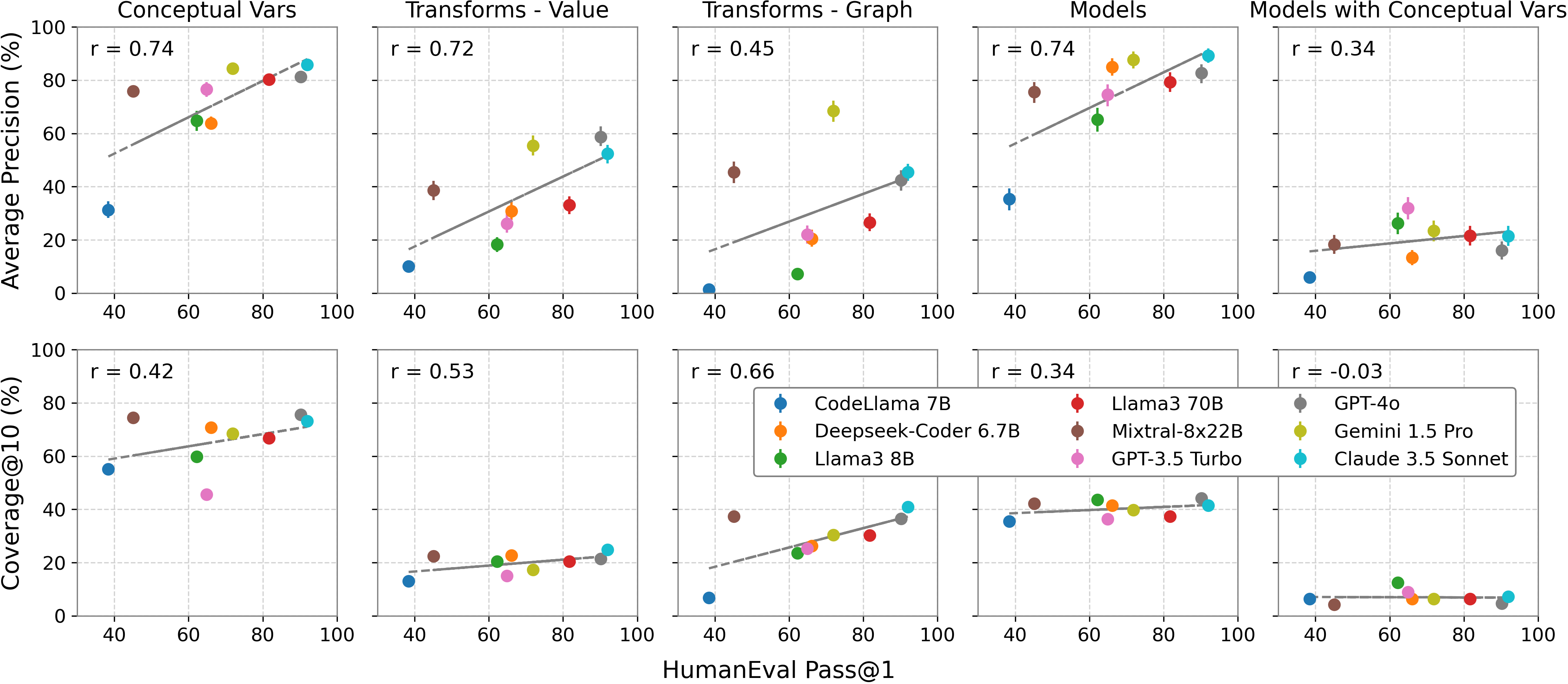
Performance vs. HumanEval Performance. We compare BLADE evaluation metrics against reported Pass@1 on HumanEval.

When comparing our results in analysis generation with those from the HumanEval coding benchmark, we fonud most metrics showed a positive correlation, indicating that higher HumanEval performance is broadly correlated with higher BLADE performance. However, coverage measures had a weaker correlation compared to precision. This suggests that while current training methods, such as Reinforcement Learning from Human Feedback (RLHF) and instruction tuning, optimize for one solution, they may struggle to generate diverse solutions.

BibTeX

@inproceedings{
  gu2024blade,
  title={BLADE: Benchmarking Language Model Agents for Data-Driven Science},
  author={Ken Gu and Ruoxi Shang and Ruien Jiang and Keying Kuang and Richard-John Lin and Donghe Lyu and Yue Mao and Youran Pan and Teng Wu and Jiaqian Yu and Yikun Zhang and Tianmai M. Zhang and Lanyi Zhu and Mike A. Merrill and Jeffrey Heer and Tim Althoff},
  booktitle={The 2024 Conference on Empirical Methods in Natural Language Processing},
  year={2024},
  }